【MATLAB数字图像处理】图像的频域处理-相位谱重构

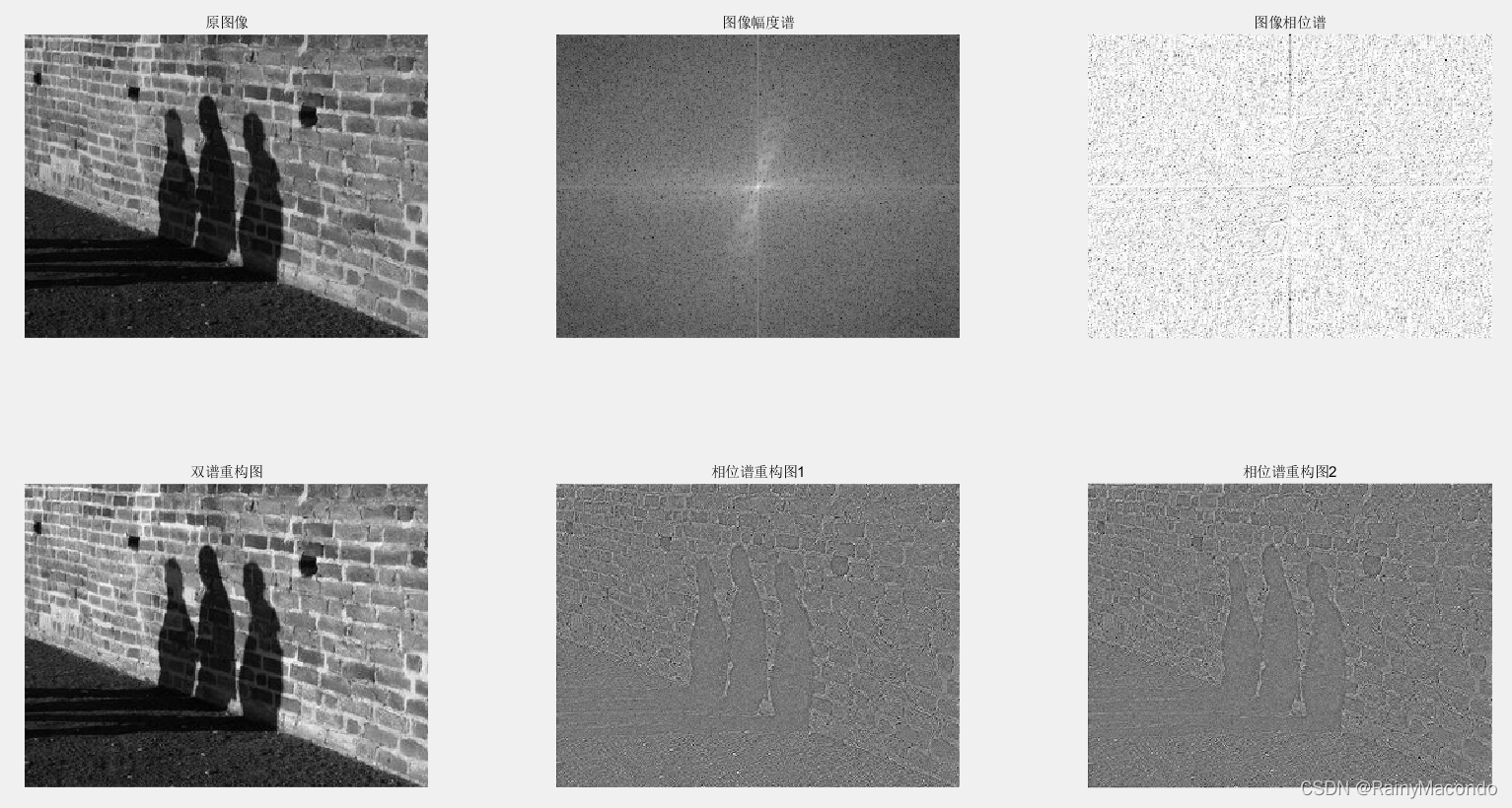
效果

%% 
clc
clear all

dir = 'image/56.jpg';

img = imread(dir);
imggray = rgb2gray(img);%灰度处理
imgf = fft2(imggray);%傅里叶变换

%对频谱进行移动，使得0频率点在中心
imgfshift = fftshift(imgf);

%获得傅里叶变换的幅度谱 
%对数变换，压缩动态范围
imgA = log(1+abs(imgfshift));

%获得傅里叶变换的相位谱
imgPhase = log(angle(imgfshift)*180/pi);

%双谱重构
imgRestructure = ifft2(abs(imgf).*exp(1i*(angle(imgf))));

%% 根据文献得到新方法：
%基于相位谱重构
%设幅度谱为常数C
c1 = 1;
c2 = 5000;
% PhaseCong = imgA .* cos(imgPhase) + imgA .* sin(imgPhase) .* 1i;
% 
% imshow(PhaseCong,[])
% imshow(imgRestructure,[])
% imgPhaseCong = abs(ifft2(PhaseCong));
imgPhaseCong1 = ifft2(abs(c1).*exp(1i*(angle(imgf))));
imgPhaseCong2 = ifft2(abs(c2).*exp(1i*(angle(imgf))));

%%
subplot(2,3,1);
imshow(imggray);
title('原图像');

subplot(2,3,2);
imshow(imgA,[]); %显示图像的幅度谱，参数'[]'是为了将其值线性拉伸
title('图像幅度谱');

subplot(2,3,3);
imshow(imgPhase,[]);
title('图像相位谱');

subplot(2,3,4);
imshow(imgRestructure,[]);
title('双谱重构图');

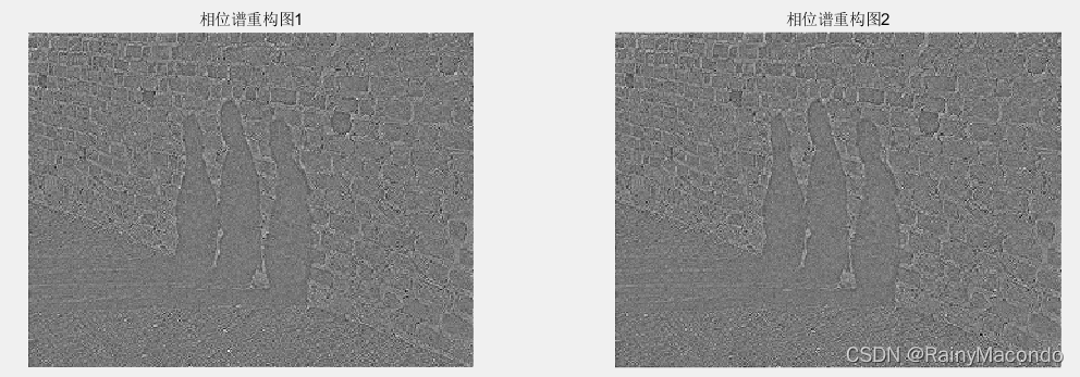
subplot(2,3,5);
imshow(imgPhaseCong1,[]);
title('相位谱重构图1');

subplot(2,3,6);
imshow(imgPhaseCong2,[]);
title('相位谱重构图2');