前言
LIO-SAM中的扫描匹配优化部分代码是直接套用LOAM,该部分代码的最大特点是没有利用任何开源的优化库(ceres-solver, g2o, gtsam…)进行残差方程的优化,而是只基于Eigen库构造了高斯牛顿迭代算法对残差方程进行优化,获得最小二乘解.一般slam后端都是基于简单易用的开源优化库进行残差方程的优化,使得代码的可读性和开发速度都得到提升,基于这样的思路,港科大基于LOAM写了一个A-LOAM框架,将里面可读性差的优化部分全部用ceres-solver优化库取代,使得代码可读性明显提高.但是,为了提升对后端残差方程优化的理解,抛弃开源优化库只利用Eigen库构造优化过程是一个非常推崇的做法.因此,对于难得的一个没有利用开源优化库进行残差方程优化的代码,对它进行剖析是非常有必要的.
扫描匹配的过程及变量定义
- 过程
当从前端传递过来当前雷达的特征点时,通过估计的雷达位姿,将特征点转换到地图坐标系下,然后通过最近邻搜索查找到转换后的特征点在地图中对应的特征,然后计算转换后特征点相对于对应特征的距离,并将此距离作为残差项进行优化. - 变量定义
x
k
+
1
,
i
L
\mathbf{x}_{k+1,i}^{L}
xk+1,iL 在时刻k+1时雷达坐标系下第i个特征点的位置(注: 特征点包括角点和面点)
x
k
+
1
,
i
W
\mathbf{x}_{k+1,i}^{W}
xk+1,iW 在时刻k+1时世界坐标系下第i个特征点的位置(通过估计的雷达位姿转换的)
T
k
+
1
W
=
[
t
x
,
t
y
,
t
z
,
r
x
,
r
y
,
r
z
]
T
\mathbf{T}_{k+1}^{W}=[tx,ty,tz,rx,ry,rz]^{T}
Tk+1W=[tx,ty,tz,rx,ry,rz]T 在时刻k+1时雷达坐标系相对于世界坐标系的变换,也即求解的目标 - 过程的公式表达(式中
x
\mathbf{x}
x为角点或者面点特征点位置坐标)
- 将雷达坐标系下特征点转换到世界坐标系下:
x
k
+
1
,
i
W
=
G
(
x
k
+
1
,
i
L
,
T
k
+
1
W
)
=
R
⋅
x
k
+
1
,
i
L
+
t
(1)
\mathbf{x}_{k+1,i}^{W} = G(\mathbf{x}_{k+1,i}^{L},\mathbf{T}_{k+1}^{W}) = \mathbf{R}\cdot\mathbf{x}_{k+1,i}^{L} + \mathbf{t} \tag{1}
xk+1,iW=G(xk+1,iL,Tk+1W)=R⋅xk+1,iL+t(1)
式中t
=
[
t
x
,
t
y
,
t
z
]
T
\mathbf{t}=[tx, ty, tz]^{T}
t=[tx,ty,tz]T,R
\mathbf{R}
R是通过欧拉角转换成的旋转矩阵,转换关系如下:
R
=
[
c
o
s
(
r
y
)
c
o
s
(
r
z
)
+
s
i
n
(
r
y
)
s
i
n
(
r
x
)
s
i
n
(
r
z
)
c
o
s
(
r
z
)
s
i
n
(
r
y
)
s
i
n
(
r
x
)
−
c
o
s
(
r
y
)
s
i
n
(
r
z
)
c
o
s
(
r
x
)
s
i
n
(
r
y
)
c
o
s
(
r
x
)
s
i
n
(
r
z
)
c
o
s
(
r
x
)
c
o
s
(
r
z
)
−
s
i
n
(
r
x
)
c
o
s
(
r
y
)
s
i
n
(
r
x
)
s
i
n
(
r
z
)
−
c
o
s
(
r
z
)
s
i
n
(
r
y
)
c
o
s
(
r
y
)
c
o
s
(
r
z
)
s
i
n
(
r
x
)
+
s
i
n
(
r
y
)
s
i
n
(
r
z
)
c
o
s
(
r
y
)
c
o
s
(
r
x
)
]
\mathbf{R} = \begin{bmatrix} cos(ry)cos(rz) + sin(ry)sin(rx)sin(rz) & cos(rz)sin(ry)sin(rx)-cos(ry)sin(rz) & cos(rx)sin(ry) \\ cos(rx)sin(rz) & cos(rx)cos(rz) & -sin(rx) \\ cos(ry)sin(rx)sin(rz)-cos(rz)sin(ry) & cos(ry)cos(rz)sin(rx)+sin(ry)sin(rz) & cos(ry)cos(rx) \end{bmatrix}
R=⎣⎡cos(ry)cos(rz)+sin(ry)sin(rx)sin(rz)cos(rx)sin(rz)cos(ry)sin(rx)sin(rz)−cos(rz)sin(ry)cos(rz)sin(ry)sin(rx)−cos(ry)sin(rz)cos(rx)cos(rz)cos(ry)cos(rz)sin(rx)+sin(ry)sin(rz)cos(rx)sin(ry)−sin(rx)cos(ry)cos(rx)⎦⎤ - 残差方程
f
=
D
(
x
k
+
1
,
i
W
,
m
)
=
D
(
G
(
x
k
+
1
,
i
L
,
T
k
+
1
W
)
,
m
)
(2)
\mathbf{f} = D(\mathbf{x}_{k+1,i}^{W}, \mathbf{m}) = D(G(\mathbf{x}_{k+1,i}^{L},\mathbf{T}_{k+1}^{W}),\mathbf{m}) \tag{2}
f=D(xk+1,iW,m)=D(G(xk+1,iL,Tk+1W),m)(2)
式中m
\mathbf{m}
m为构建的局部关键帧地图.
优化过程分析
LIO-SAM中采用的是高斯牛顿迭代法进行残差方程的优化,该迭代法迭代公式如下:
J
T
J
⋅
Δ
T
=
−
J
T
f
(3)
\mathbf{J}^{T}\mathbf{J}\cdot\Delta T = -\mathbf{J}^{T}\mathbf{f} \tag{3}
JTJ⋅ΔT=−JTf(3)
式中
J
\mathbf{J}
J为残差方程相对于优化变量的雅克比矩阵,
f
\mathbf{f}
f为残差方程结果,
Δ
T
\Delta T
ΔT为优化变量增量.根据公式(2)的残差方程定义,可采用链式法则求得雅克比矩阵
J
\mathbf{J}
J,计算公式如下:
J
=
∂
f
∂
T
k
+
1
W
=
∂
D
(
⋅
)
∂
G
(
⋅
)
⋅
∂
G
(
⋅
)
∂
T
k
+
1
W
(4)
\mathbf{J} = \frac{\partial{\mathbf{f}}}{\partial{\mathbf{T}_{k+1}^{W}}} = \frac{\partial{D(\cdot)}}{\partial{G(\cdot)}} \cdot \frac{\partial{G(\cdot)}}{\partial{\mathbf{T}_{k+1}^{W}}} \tag{4}
J=∂Tk+1W∂f=∂G(⋅)∂D(⋅)⋅∂Tk+1W∂G(⋅)(4)
将
J
\mathbf{J}
J分成两部分
J
=
[
J
t
,
J
r
]
T
\mathbf{J}=[\mathbf{J}_{\mathbf{t}},\mathbf{J}_{\mathbf{r}}]^{T}
J=[Jt,Jr]T,分别为残差方程相对于优化变量平移部分
t
=
[
t
x
,
t
y
,
t
z
]
T
\mathbf{t}=[tx, ty, tz]^{T}
t=[tx,ty,tz]T的和旋转部分
r
=
[
r
x
,
r
y
,
r
z
]
T
\mathbf{r}=[rx,ry,rz]^{T}
r=[rx,ry,rz]T的雅克比矩阵.于是可以将式(4)拆分成下面两部分:
J
t
=
∂
D
(
⋅
)
∂
G
(
⋅
)
⋅
∂
G
(
⋅
)
∂
t
k
+
1
W
=
∂
D
(
⋅
)
∂
G
(
⋅
)
(5)
\mathbf{J_{t}} = \frac{\partial{D(\cdot)}}{\partial{G(\cdot)}} \cdot \frac{\partial{G(\cdot)}}{\partial{\mathbf{t}_{k+1}^{W}}}= \frac{\partial{D(\cdot)}}{\partial{G(\cdot)}} \tag{5}
Jt=∂G(⋅)∂D(⋅)⋅∂tk+1W∂G(⋅)=∂G(⋅)∂D(⋅)(5)
J
r
=
∂
D
(
⋅
)
∂
G
(
⋅
)
⋅
∂
G
(
⋅
)
∂
r
k
+
1
W
=
∂
D
(
⋅
)
∂
G
(
⋅
)
⋅
∂
R
k
+
1
W
∂
r
k
+
1
W
⋅
x
k
+
1
,
i
L
(6)
\mathbf{J_{r}} = \frac{\partial{D(\cdot)}}{\partial{G(\cdot)}} \cdot \frac{\partial{G(\cdot)}}{\partial{\mathbf{r}_{k+1}^{W}}} = \frac{\partial{D(\cdot)}}{\partial{G(\cdot)}} \cdot \frac{\partial{\mathbf{R}_{k+1}^{W}}}{\partial{\mathbf{r}_{k+1}^{W}}}\cdot \mathbf{x}_{k+1,i}^{L} \tag{6}
Jr=∂G(⋅)∂D(⋅)⋅∂rk+1W∂G(⋅)=∂G(⋅)∂D(⋅)⋅∂rk+1W∂Rk+1W⋅xk+1,iL(6)
公式(6)又可以进一步分解为
J
r
=
[
J
r
x
,
J
r
y
,
J
r
z
]
T
\mathbf{J_{r}}=[\mathbf{J}_{rx}, \mathbf{J}_{ry}, \mathbf{J}_{rz}]^{T}
Jr=[Jrx,Jry,Jrz]T三部分,对应公式如下:
J
r
x
=
∂
D
(
⋅
)
∂
G
(
⋅
)
⋅
∂
R
k
+
1
W
∂
(
r
x
)
k
+
1
W
⋅
x
k
+
1
,
i
L
=
∂
D
(
⋅
)
∂
G
(
⋅
)
⋅
[
s
i
n
(
r
y
)
c
o
s
(
r
x
)
s
i
n
(
r
z
)
c
o
s
(
r
z
)
s
i
n
(
r
y
)
c
o
s
(
r
x
)
−
s
i
n
(
r
x
)
s
i
n
(
r
y
)
−
s
i
n
(
r
x
)
s
i
n
(
r
z
)
−
s
i
n
(
r
x
)
c
o
s
(
r
z
)
−
c
o
s
(
r
x
)
c
o
s
(
r
y
)
c
o
s
(
r
x
)
s
i
n
(
r
z
)
c
o
s
(
r
y
)
c
o
s
(
r
z
)
c
o
s
(
r
x
)
−
c
o
s
(
r
y
)
s
i
n
(
r
x
)
]
⋅
x
k
+
1
,
i
L
(7)
\begin{aligned} \mathbf{J}_{rx}&=\frac{\partial{D(\cdot)}}{\partial{G(\cdot)}} \cdot \frac{\partial{\mathbf{R}_{k+1}^{W}}}{\partial{{(rx)}_{k+1}^{W}}}\cdot \mathbf{x}_{k+1,i}^{L} \\ &=\frac{\partial{D(\cdot)}}{\partial{G(\cdot)}} \cdot \begin{bmatrix} sin(ry)cos(rx)sin(rz) & cos(rz)sin(ry)cos(rx) & -sin(rx)sin(ry) \\ -sin(rx)sin(rz) & -sin(rx)cos(rz) & -cos(rx) \\ cos(ry)cos(rx)sin(rz) & cos(ry)cos(rz)cos(rx) & -cos(ry)sin(rx) \end{bmatrix} \cdot \mathbf{x}_{k+1,i}^{L} \end{aligned} \tag{7}
Jrx=∂G(⋅)∂D(⋅)⋅∂(rx)k+1W∂Rk+1W⋅xk+1,iL=∂G(⋅)∂D(⋅)⋅⎣⎡sin(ry)cos(rx)sin(rz)−sin(rx)sin(rz)cos(ry)cos(rx)sin(rz)cos(rz)sin(ry)cos(rx)−sin(rx)cos(rz)cos(ry)cos(rz)cos(rx)−sin(rx)sin(ry)−cos(rx)−cos(ry)sin(rx)⎦⎤⋅xk+1,iL(7)
J
r
y
=
∂
D
(
⋅
)
∂
G
(
⋅
)
⋅
∂
R
k
+
1
W
∂
(
r
y
)
k
+
1
W
⋅
x
k
+
1
,
i
L
=
∂
D
(
⋅
)
∂
G
(
⋅
)
⋅
[
−
s
i
n
(
r
y
)
c
o
s
(
r
z
)
+
c
o
s
(
r
y
)
s
i
n
(
r
x
)
s
i
n
(
r
z
)
c
o
s
(
r
z
)
c
o
s
(
r
y
)
s
i
n
(
r
x
)
+
s
i
n
(
r
y
)
s
i
n
(
r
z
)
c
o
s
(
r
x
)
c
o
s
(
r
y
)
0
0
0
−
s
i
n
(
r
y
)
s
i
n
(
r
x
)
s
i
n
(
r
z
)
−
c
o
s
(
r
z
)
c
o
s
(
r
y
)
−
s
i
n
(
r
y
)
c
o
s
(
r
z
)
s
i
n
(
r
x
)
+
c
o
s
(
r
y
)
s
i
n
(
r
z
)
−
s
i
n
(
r
y
)
c
o
s
(
r
x
)
]
⋅
x
k
+
1
,
i
L
(8)
\begin{aligned} \mathbf{J}_{ry}&=\frac{\partial{D(\cdot)}}{\partial{G(\cdot)}} \cdot \frac{\partial{\mathbf{R}_{k+1}^{W}}}{\partial{{(ry)}_{k+1}^{W}}}\cdot \mathbf{x}_{k+1,i}^{L} \\ &=\frac{\partial{D(\cdot)}}{\partial{G(\cdot)}} \cdot \begin{bmatrix} -sin(ry)cos(rz)+cos(ry)sin(rx)sin(rz) & cos(rz)cos(ry)sin(rx)+sin(ry)sin(rz) & cos(rx)cos(ry) \\ 0 & 0 & 0 \\ -sin(ry)sin(rx)sin(rz)-cos(rz)cos(ry) & -sin(ry)cos(rz)sin(rx)+cos(ry)sin(rz) & -sin(ry)cos(rx) \end{bmatrix} \cdot \mathbf{x}_{k+1,i}^{L} \end{aligned} \tag{8}
Jry=∂G(⋅)∂D(⋅)⋅∂(ry)k+1W∂Rk+1W⋅xk+1,iL=∂G(⋅)∂D(⋅)⋅⎣⎡−sin(ry)cos(rz)+cos(ry)sin(rx)sin(rz)0−sin(ry)sin(rx)sin(rz)−cos(rz)cos(ry)cos(rz)cos(ry)sin(rx)+sin(ry)sin(rz)0−sin(ry)cos(rz)sin(rx)+cos(ry)sin(rz)cos(rx)cos(ry)0−sin(ry)cos(rx)⎦⎤⋅xk+1,iL(8)
J
r
z
=
∂
D
(
⋅
)
∂
G
(
⋅
)
⋅
∂
R
k
+
1
W
∂
(
r
z
)
k
+
1
W
⋅
x
k
+
1
,
i
L
=
∂
D
(
⋅
)
∂
G
(
⋅
)
⋅
[
−
c
o
s
(
r
y
)
s
i
n
(
r
z
)
+
s
i
n
(
r
y
)
s
i
n
(
r
x
)
c
o
s
(
r
z
)
−
s
i
n
(
r
z
)
s
i
n
(
r
y
)
s
i
n
(
r
x
)
−
c
o
s
(
r
y
)
c
o
s
(
r
z
)
0
c
o
s
(
r
x
)
c
o
s
(
r
z
)
−
c
o
s
(
r
x
)
s
i
n
(
r
z
)
0
c
o
s
(
r
y
)
s
i
n
(
r
x
)
c
o
s
(
r
z
)
+
s
i
n
(
r
z
)
s
i
n
(
r
y
)
−
c
o
s
(
r
y
)
s
i
n
(
r
z
)
s
i
n
(
r
x
)
+
s
i
n
(
r
y
)
c
o
s
(
r
z
)
0
]
⋅
x
k
+
1
,
i
L
(9)
\begin{aligned} \mathbf{J}_{rz}&=\frac{\partial{D(\cdot)}}{\partial{G(\cdot)}} \cdot \frac{\partial{\mathbf{R}_{k+1}^{W}}}{\partial{{(rz)}_{k+1}^{W}}}\cdot \mathbf{x}_{k+1,i}^{L} \\ &=\frac{\partial{D(\cdot)}}{\partial{G(\cdot)}} \cdot \begin{bmatrix} -cos(ry)sin(rz)+sin(ry)sin(rx)cos(rz) & -sin(rz)sin(ry)sin(rx)-cos(ry)cos(rz) & 0\\ cos(rx)cos(rz) & -cos(rx)sin(rz) & 0 \\ cos(ry)sin(rx)cos(rz)+sin(rz)sin(ry) & -cos(ry)sin(rz)sin(rx)+sin(ry)cos(rz) & 0 \end{bmatrix} \cdot \mathbf{x}_{k+1,i}^{L} \end{aligned} \tag{9}
Jrz=∂G(⋅)∂D(⋅)⋅∂(rz)k+1W∂Rk+1W⋅xk+1,iL=∂G(⋅)∂D(⋅)⋅⎣⎡−cos(ry)sin(rz)+sin(ry)sin(rx)cos(rz)cos(rx)cos(rz)cos(ry)sin(rx)cos(rz)+sin(rz)sin(ry)−sin(rz)sin(ry)sin(rx)−cos(ry)cos(rz)−cos(rx)sin(rz)−cos(ry)sin(rz)sin(rx)+sin(ry)cos(rz)000⎦⎤⋅xk+1,iL(9)
通过以上分析过程可知,要想进行高斯牛顿迭代方法求解关键帧位姿,还需要确定残差方程
f
\mathbf{f}
f来计算残差结果,并且基于残差方程计算雅克比矩阵中的
∂
D
(
⋅
)
∂
G
(
⋅
)
\frac{\partial{D(\cdot)}}{\partial{G(\cdot)}}
∂G(⋅)∂D(⋅)项.
角点特征点残差方程构建
(1) 残差方程的构建
LOAM论文中对角点特征点残差方程定义如下:
d
ε
=
∣
(
x
~
k
+
1
,
i
W
−
x
ˉ
k
,
j
W
)
×
(
x
~
k
+
1
,
i
W
−
x
ˉ
k
,
l
W
)
∣
∣
(
x
ˉ
k
,
j
W
−
x
ˉ
k
,
l
W
)
∣
(10)
d_{\varepsilon} = \frac{\left| (\widetilde{\mathbf{x}}_{k+1,i}^{W}-\bar{\mathbf{x}}_{k,j}^{W}) \times (\widetilde{\mathbf{x}}_{k+1,i}^{W}-\bar{\mathbf{x}}_{k,l}^{W}) \right|} {\left| (\bar{\mathbf{x}}_{k,j}^{W}-\bar{\mathbf{x}}_{k,l}^{W}) \right|} \tag{10}
dε=∣∣∣(xˉk,jW−xˉk,lW)∣∣∣∣∣∣(x
k+1,iW−xˉk,jW)×(x
k+1,iW−xˉk,lW)∣∣∣(10)
式中
x
~
k
+
1
,
i
W
\widetilde{\mathbf{x}}_{k+1,i}^{W}
x
k+1,iW表示在k+1时刻第i个特征点通过估计的雷达位姿转换到世界坐标系下的特征点坐标,
x
ˉ
k
,
j
W
\bar{\mathbf{x}}_{k,j}^{W}
xˉk,jW和
x
ˉ
k
,
l
W
\bar{\mathbf{x}}_{k,l}^{W}
xˉk,lW分别表示第i个角点特征点在地图中对应的边线特征上的两个坐标点.该公式的原理可用下图进行说明.
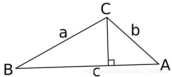
推导:
S
Δ
A
B
C
=
1
2
a
∗
b
∗
s
i
n
(
C
)
S
Δ
A
B
C
=
1
2
c
∗
h
∵
∣
a
×
b
∣
=
a
∗
b
∗
s
i
n
(
C
)
∴
h
=
∣
a
×
b
∣
∣
c
∣
\begin{aligned} S\Delta ABC &= \frac{1}{2}a*b*sin(C)\\ S\Delta ABC &= \frac{1}{2}c*h\\ \because \left| \mathbf{a}\times\mathbf{b} \right| &= a*b*sin(C)\\ \therefore h &= \frac{\left| \mathbf{a}\times\mathbf{b} \right|}{\left| \mathbf{c} \right|} \end{aligned}
SΔABCSΔABC∵∣a×b∣∴h=21a∗b∗sin(C)=21c∗h=a∗b∗sin(C)=∣c∣∣a×b∣
(2)
∂
D
(
⋅
)
∂
G
(
⋅
)
\frac{\partial{D(\cdot)}}{\partial{G(\cdot)}}
∂G(⋅)∂D(⋅)求解
为了与代码一致,定义公式(10)中的变量
x
~
k
+
1
,
i
W
=
[
x
0
,
y
0
,
z
0
]
T
,
x
ˉ
k
,
j
W
=
[
x
1
,
y
1
,
z
1
]
T
,
x
ˉ
k
,
l
W
=
[
x
2
,
y
2
,
z
2
]
T
\widetilde{\mathbf{x}}_{k+1,i}^{W}=[x_{0}, y_{0}, z_{0}]^{T}, \bar{\mathbf{x}}_{k,j}^{W}=[x_{1},y_{1},z_{1}]^{T},\bar{\mathbf{x}}_{k,l}^{W}=[x_{2},y_{2},z_{2}]^{T}
x
k+1,iW=[x0,y0,z0]T,xˉk,jW=[x1,y1,z1]T,xˉk,lW=[x2,y2,z2]T 基于此定义,对方程(10)进行展开:
d
ε
=
a
012
l
12
=
∣
[
(
y
0
−
y
1
)
(
z
0
−
z
2
)
−
(
z
0
−
z
1
)
(
y
0
−
y
2
)
(
z
0
−
z
1
)
(
x
0
−
x
2
)
−
(
x
0
−
x
1
)
(
z
0
−
z
2
)
(
x
0
−
x
1
)
(
y
0
−
y
2
)
−
(
y
0
−
y
1
)
(
x
0
−
x
2
)
]
∣
∣
[
(
x
1
−
x
2
)
(
y
1
−
y
2
)
(
z
1
−
z
2
)
]
∣
=
[
(
y
0
−
y
1
)
(
z
0
−
z
2
)
−
(
z
0
−
z
1
)
(
y
0
−
y
2
)
]
2
+
[
(
z
0
−
z
1
)
(
x
0
−
x
2
)
−
(
x
0
−
x
1
)
(
z
0
−
z
2
)
]
2
+
[
(
x
0
−
x
1
)
(
y
0
−
y
2
)
−
(
y
0
−
y
1
)
(
x
0
−
x
2
)
]
2
(
x
1
−
x
2
)
2
+
(
y
1
−
y
2
)
2
+
(
z
1
−
z
2
)
2
(11)
\begin{aligned} d_{\varepsilon} &=\frac{a_{012}}{l_{12}} = \frac{\left| \begin{bmatrix} (y0-y1)(z0-z2)-(z0-z1)(y0-y2)\\ (z0-z1)(x0-x2)-(x0-x1)(z0-z2)\\ (x0-x1)(y0-y2)-(y0-y1)(x0-x2) \end{bmatrix} \right|}{\left| \begin{bmatrix} (x1-x2)\\ (y1-y2)\\ (z1-z2) \end{bmatrix} \right|} \\ &=\frac{\sqrt{[(y0-y1)(z0-z2)-(z0-z1)(y0-y2)]^2 + [(z0-z1)(x0-x2)-(x0-x1)(z0-z2)]^2+[(x0-x1)(y0-y2)-(y0-y1)(x0-x2)]^2}} {\sqrt{(x1-x2)^{2}+(y1-y2)^{2}+(z1-z2)^{2}}} \end{aligned} \tag{11}
dε=l12a012=∣∣∣∣∣∣⎣⎡(x1−x2)(y1−y2)(z1−z2)⎦⎤∣∣∣∣∣∣∣∣∣∣∣∣⎣⎡(y0−y1)(z0−z2)−(z0−z1)(y0−y2)(z0−z1)(x0−x2)−(x0−x1)(z0−z2)(x0−x1)(y0−y2)−(y0−y1)(x0−x2)⎦⎤∣∣∣∣∣∣=(x1−x2)2+(y1−y2)2+(z1−z2)2[(y0−y1)(z0−z2)−(z0−z1)(y0−y2)]2+[(z0−z1)(x0−x2)−(x0−x1)(z0−z2)]2+[(x0−x1)(y0−y2)−(y0−y1)(x0−x2)]2(11)
所以有:
∂
D
(
⋅
)
∂
G
(
⋅
)
=
[
l
a
l
b
l
c
]
=
∂
d
ε
∂
x
~
k
+
1
,
i
W
=
[
∂
d
ε
∂
x
0
,
∂
d
ε
∂
x
1
,
∂
d
ε
∂
x
2
]
T
=
[
(
(
y
1
−
y
2
)
(
(
x
0
−
x
1
)
(
y
0
−
y
2
)
−
(
x
0
−
x
2
)
(
y
0
−
y
1
)
)
+
(
z
1
−
z
2
)
(
(
x
0
−
x
1
)
(
z
0
−
z
2
)
−
(
x
0
−
x
2
)
(
z
0
−
z
1
)
)
)
/
a
012
/
l
12
−
(
(
x
1
−
x
2
)
(
(
x
0
−
x
1
)
(
y
0
−
y
2
)
−
(
x
0
−
x
2
)
(
y
0
−
y
1
)
)
−
(
z
1
−
z
2
)
(
(
y
0
−
y
1
)
(
z
0
−
z
2
)
−
(
y
0
−
y
2
)
(
z
0
−
z
1
)
)
)
/
a
012
/
l
12
−
(
(
x
1
−
x
2
)
(
(
x
0
−
x
1
)
(
z
0
−
z
2
)
−
(
x
0
−
x
2
)
(
z
0
−
z
1
)
)
+
(
y
1
−
y
2
)
(
(
y
0
−
y
1
)
(
z
0
−
z
2
)
−
(
y
0
−
y
2
)
(
z
0
−
z
1
)
)
)
/
a
012
/
l
12
]
(12)
\begin{aligned} \frac{\partial{D(\cdot)}}{\partial{G(\cdot)}} &= \begin{bmatrix} la \\ lb \\ lc \end{bmatrix}=\frac{\partial d_{\varepsilon}}{\partial{\widetilde{\mathbf{x}}_{k+1,i}^{W}}} = [\frac{\partial{d_{\varepsilon}}}{\partial{x0}}, \frac{\partial{d_{\varepsilon}}}{\partial{x1}}, \frac{\partial{d_{\varepsilon}}}{\partial{x2}}]^{T} \\ &= \begin{bmatrix} ((y1 – y2)((x0 – x1)(y0 – y2) – (x0 – x2)(y0 – y1)) + (z1 – z2)((x0 – x1)(z0 – z2) – (x0 – x2)(z0 – z1))) / a012 / l12\\ -((x1 – x2)((x0 – x1)(y0 – y2) – (x0 – x2)(y0 – y1)) – (z1 – z2)((y0 – y1)(z0 – z2) – (y0 – y2)(z0 – z1))) / a012 / l12\\ -((x1 – x2)((x0 – x1)(z0 – z2) – (x0 – x2)(z0 – z1)) + (y1 – y2)((y0 – y1)(z0 – z2) – (y0 – y2)(z0 – z1))) / a012 / l12 \end{bmatrix} \end{aligned} \tag{12}
∂G(⋅)∂D(⋅)=⎣⎡lalblc⎦⎤=∂x
k+1,iW∂dε=[∂x0∂dε,∂x1∂dε,∂x2∂dε]T=⎣⎡((y1−y2)((x0−x1)(y0−y2)−(x0−x2)(y0−y1))+(z1−z2)((x0−x1)(z0−z2)−(x0−x2)(z0−z1)))/a012/l12−((x1−x2)((x0−x1)(y0−y2)−(x0−x2)(y0−y1))−(z1−z2)((y0−y1)(z0−z2)−(y0−y2)(z0−z1)))/a012/l12−((x1−x2)((x0−x1)(z0−z2)−(x0−x2)(z0−z1))+(y1−y2)((y0−y1)(z0−z2)−(y0−y2)(z0−z1)))/a012/l12⎦⎤(12)
面点特征点残差方程构建
(1) 残差方程的构建
此部分代码与论文LOAM论文中提供的公式(3)有些不一样,我们这里以代码为准进行说明.代码中首先利用面点地图中与面特征点最近的5个特征点构建超定方程,然后通过QR分解计算面特征点对应的面特征
p
a
⋅
x
+
p
b
⋅
y
+
p
c
⋅
z
+
p
d
=
0
pa\cdot x + pb\cdot y + pc\cdot z + pd = 0
pa⋅x+pb⋅y+pc⋅z+pd=0.基于此面特征构建的面特征点残差方程如下:
d
H
=
p
a
⋅
x
+
p
b
⋅
y
+
p
c
⋅
z
+
p
d
p
a
2
+
p
b
2
+
p
c
2
(13)
d_{H} = \frac{pa\cdot x + pb\cdot y + pc\cdot z + pd}{\sqrt{pa^{2}+pb^{2}+pc^{2}}} \tag{13}
dH=pa2+pb2+pc2pa⋅x+pb⋅y+pc⋅z+pd(13)
式中
x
=
[
x
,
y
,
z
]
T
\mathbf{x} = [x, y, z]^{T}
x=[x,y,z]T表示雷达坐标系下的面特征点通过估计的雷达位姿转换到世界坐标系下的坐标.
(2)
∂
D
(
⋅
)
∂
G
(
⋅
)
\frac{\partial{D(\cdot)}}{\partial{G(\cdot)}}
∂G(⋅)∂D(⋅)求解
令
p
s
=
p
a
2
+
p
b
2
+
p
c
2
ps = \sqrt{pa^{2}+pb^{2}+pc^{2}}
ps=pa2+pb2+pc2得:
∂
D
(
⋅
)
∂
G
(
⋅
)
=
∂
d
H
∂
x
=
[
∂
d
H
∂
x
,
∂
d
H
∂
y
,
∂
d
H
∂
z
]
T
=
[
p
a
/
p
s
,
p
b
/
p
s
,
p
c
/
p
s
,
p
d
/
p
s
]
T
(14)
\begin{aligned} \frac{\partial{D(\cdot)}}{\partial{G(\cdot)}} &= \frac{\partial d_{H}}{\partial \mathbf{x}}=[\frac{\partial d_{H}}{\partial x},\frac{\partial d_{H}}{\partial y},\frac{\partial d_{H}}{\partial z}]^{T} \\ &= [pa/ps, pb/ps, pc/ps, pd/ps]^{T} \end{aligned} \tag{14}
∂G(⋅)∂D(⋅)=∂x∂dH=[∂x∂dH,∂y∂dH,∂z∂dH]T=[pa/ps,pb/ps,pc/ps,pd/ps]T(14)
代码解析
(1) 角点特征点残差方程的构建
void cornerOptimization()
{
    updatePointAssociateToMap();

    for (int i = 0; i < laserCloudCornerLastDSNum; i++)
    {
        PointType pointOri, pointSel, coeff;
        std::vector<int> pointSearchInd;
        std::vector<float> pointSearchSqDis;

        pointOri = laserCloudCornerLastDS->points[i];
        pointAssociateToMap(&pointOri, &pointSel); // 将雷达坐标系下的角特征点转换到世界坐标系下
        kdtreeCornerFromMap->nearestKSearch(pointSel, 5, pointSearchInd, pointSearchSqDis); // 在角特征点地图中寻找最近的五个角特征点

        cv::Mat matA1(3, 3, CV_32F, cv::Scalar::all(0));
        cv::Mat matD1(1, 3, CV_32F, cv::Scalar::all(0));
        cv::Mat matV1(3, 3, CV_32F, cv::Scalar::all(0));

        if (pointSearchSqDis[4] < 1.0)
        {
            // 计算最近5个点的中心坐标
            float cx = 0, cy = 0, cz = 0;
            for (int j = 0; j < 5; j++)
            {
                cx += laserCloudCornerFromMapDS->points[pointSearchInd[j]].x;
                cy += laserCloudCornerFromMapDS->points[pointSearchInd[j]].y;
                cz += laserCloudCornerFromMapDS->points[pointSearchInd[j]].z;
            }
            cx /= 5;
            cy /= 5;
            cz /= 5;

            // 计算5个点相对于中心点分布的协方差
            float a11 = 0, a12 = 0, a13 = 0, a22 = 0, a23 = 0, a33 = 0;
            for (int j = 0; j < 5; j++)
            {
                float ax = laserCloudCornerFromMapDS->points[pointSearchInd[j]].x - cx;
                float ay = laserCloudCornerFromMapDS->points[pointSearchInd[j]].y - cy;
                float az = laserCloudCornerFromMapDS->points[pointSearchInd[j]].z - cz;

                a11 += ax * ax;
                a12 += ax * ay;
                a13 += ax * az;
                a22 += ay * ay;
                a23 += ay * az;
                a33 += az * az;
            }
            a11 /= 5;
            a12 /= 5;
            a13 /= 5;
            a22 /= 5;
            a23 /= 5;
            a33 /= 5;

            // 协方差矩阵
            matA1.at<float>(0, 0) = a11;
            matA1.at<float>(0, 1) = a12;
            matA1.at<float>(0, 2) = a13;
            matA1.at<float>(1, 0) = a12;
            matA1.at<float>(1, 1) = a22;
            matA1.at<float>(1, 2) = a23;
            matA1.at<float>(2, 0) = a13;
            matA1.at<float>(2, 1) = a23;
            matA1.at<float>(2, 2) = a33;

            // 计算协方差矩阵的特征值和特征向量
            cv::eigen(matA1, matD1, matV1);

            // 由于cv::eigen获得的特征值是按从大到小的顺序排列的,因此,此处表示的是存在一个特征值明显大于其它特征值
            // 最大特征值matD1.at<float>(0,0)对应的特征向量matV1.at<float>(0)为特征直线的方向
            if (matD1.at<float>(0, 0) > 3 * matD1.at<float>(0, 1))
            {
                // 当前待匹配角特征点,对应公式(10)中x_{k+1,i}_w
                float x0 = pointSel.x;
                float y0 = pointSel.y;
                float z0 = pointSel.z;
                // 局部地图中对应的特征直线上的两点坐标
                // 对应公式(10)中x_{k,j}_w
                float x1 = cx + 0.1 * matV1.at<float>(0, 0);
                float y1 = cy + 0.1 * matV1.at<float>(0, 1);
                float z1 = cz + 0.1 * matV1.at<float>(0, 2);
                // 对应公式(10)中x_{k,l}_w
                float x2 = cx - 0.1 * matV1.at<float>(0, 0);
                float y2 = cy - 0.1 * matV1.at<float>(0, 1);
                float z2 = cz - 0.1 * matV1.at<float>(0, 2);

                // 对应公式(11)中的a012
                float a012 = sqrt(((x0 - x1) * (y0 - y2) - (x0 - x2) * (y0 - y1)) * ((x0 - x1) * (y0 - y2) - (x0 - x2) * (y0 - y1)) + ((x0 - x1) * (z0 - z2) - (x0 - x2) * (z0 - z1)) * ((x0 - x1) * (z0 - z2) - (x0 - x2) * (z0 - z1)) + ((y0 - y1) * (z0 - z2) - (y0 - y2) * (z0 - z1)) * ((y0 - y1) * (z0 - z2) - (y0 - y2) * (z0 - z1)));
                // 对应公式(11)中的l12
                float l12 = sqrt((x1 - x2) * (x1 - x2) + (y1 - y2) * (y1 - y2) + (z1 - z2) * (z1 - z2));
                // 对应公式(12)中的la
                float la = ((y1 - y2) * ((x0 - x1) * (y0 - y2) - (x0 - x2) * (y0 - y1)) + (z1 - z2) * ((x0 - x1) * (z0 - z2) - (x0 - x2) * (z0 - z1))) / a012 / l12;
                // 对应公式(12)中的lb
                float lb = -((x1 - x2) * ((x0 - x1) * (y0 - y2) - (x0 - x2) * (y0 - y1)) - (z1 - z2) * ((y0 - y1) * (z0 - z2) - (y0 - y2) * (z0 - z1))) / a012 / l12;
                // 对应公式(12)中的lc
                float lc = -((x1 - x2) * ((x0 - x1) * (z0 - z2) - (x0 - x2) * (z0 - z1)) + (y1 - y2) * ((y0 - y1) * (z0 - z2) - (y0 - y2) * (z0 - z1))) / a012 / l12;
                // 对应公式(10)中的d_e
                float ld2 = a012 / l12;
                // 计算权重(距离越远,权重越小,相当于损失函数,为了抑制噪声的影响)
                float s = 1 - 0.9 * fabs(ld2);
                // [coeff.x, coeff.y, coeff.z]对应公式(12)中的 partial_D / partial_G
                coeff.x = s * la;
                coeff.y = s * lb;
                coeff.z = s * lc;
                // coeff.intensity保存残差方程的残差值,对应公式(10)中的 d_e
                coeff.intensity = s * ld2;

                if (s > 0.1)
                {
                    laserCloudOriCornerVec[i] = pointOri;
                    coeffSelCornerVec[i] = coeff;
                    laserCloudOriCornerFlag[i] = true;
                }
            }
        }
    }
}
(2) 面点特征点残差方程构建
void surfOptimization()
{
    updatePointAssociateToMap();
    for (int i = 0; i < laserCloudSurfLastDSNum; i++)
    {
        PointType pointOri, pointSel, coeff;
        std::vector<int> pointSearchInd;
        std::vector<float> pointSearchSqDis;

        pointOri = laserCloudSurfLastDS->points[i];
        pointAssociateToMap(&pointOri, &pointSel); //将雷达坐标系下的面特征点转换到世界坐标系下
        kdtreeSurfFromMap->nearestKSearch(pointSel, 5, pointSearchInd, pointSearchSqDis); // 在角特征点地图中寻找最近的五个面特征点

        Eigen::Matrix<float, 5, 3> matA0;
        Eigen::Matrix<float, 5, 1> matB0;
        Eigen::Vector3f matX0;

        matA0.setZero();
        matB0.fill(-1);
        matX0.setZero();

        if (pointSearchSqDis[4] < 1.0)
        {
            // 利用5个平面点构建超定方程,并利用qr分解计算拟合的平面系数
            for (int j = 0; j < 5; j++)
            {
                matA0(j, 0) = laserCloudSurfFromMapDS->points[pointSearchInd[j]].x;
                matA0(j, 1) = laserCloudSurfFromMapDS->points[pointSearchInd[j]].y;
                matA0(j, 2) = laserCloudSurfFromMapDS->points[pointSearchInd[j]].z;
            }

            matX0 = matA0.colPivHouseholderQr().solve(matB0);

            // 平面系数ax+by+cz+1=0
            float pa = matX0(0, 0);
            float pb = matX0(1, 0);
            float pc = matX0(2, 0);
            float pd = 1;

            // 对应公式(14)中的偏导数 partial_D / partial_G
            float ps = sqrt(pa * pa + pb * pb + pc * pc);
            pa /= ps;
            pb /= ps;
            pc /= ps;
            pd /= ps;

            bool planeValid = true;
            for (int j = 0; j < 5; j++)
            {
                if (fabs(pa * laserCloudSurfFromMapDS->points[pointSearchInd[j]].x +
                         pb * laserCloudSurfFromMapDS->points[pointSearchInd[j]].y +
                         pc * laserCloudSurfFromMapDS->points[pointSearchInd[j]].z + pd) > 0.2)
                {
                    planeValid = false;
                    break;
                }
            }

            if (planeValid)
            {
                // 计算当前特征点到目标平面特征的距离,即残差值,对应公式(13)中的d_H
                float pd2 = pa * pointSel.x + pb * pointSel.y + pc * pointSel.z + pd;

                // 计算权重(残差值越大,权重越小,相当于损失函数,抑制噪声影响)
                float s = 1 - 0.9 * fabs(pd2) / sqrt(sqrt(pointSel.x * pointSel.x + pointSel.y * pointSel.y + pointSel.z * pointSel.z));
				 // [coeff.x, coeff.y, coeff.z]对应公式(14)中的 partial_D / partial_G
                coeff.x = s * pa;
                coeff.y = s * pb;
                coeff.z = s * pc;
                // coeff.intensity保存残差方程的残差值,对应公式(13)中的 d_e
                coeff.intensity = s * pd2;

                if (s > 0.1)
                {
                    laserCloudOriSurfVec[i] = pointOri;
                    coeffSelSurfVec[i] = coeff;
                    laserCloudOriSurfFlag[i] = true;
                }
            }
        }
    }
}
(3) 高斯牛顿迭代优化过程
bool LMOptimization(int iterCount)
{
    // lidar -> camera
    float srx = sin(transformTobeMapped[1]); // 对应上面原理部分的sin(rx)
    float crx = cos(transformTobeMapped[1]); // 对应上面原理部分的cos(rx)
    float sry = sin(transformTobeMapped[2]); // 对应上面原理部分的sin(ry)
    float cry = cos(transformTobeMapped[2]); // 对应上面原理部分的cos(ry)
    float srz = sin(transformTobeMapped[0]); // 对应上面原理部分的sin(rz)
    float crz = cos(transformTobeMapped[0]); // 对应上面原理部分的cos(rz)

    int laserCloudSelNum = laserCloudOri->size();
    if (laserCloudSelNum < 50)
    {
        return false;
    }

    cv::Mat matA(laserCloudSelNum, 6, CV_32F, cv::Scalar::all(0)); // 对应公式(3)中的雅克比矩阵J
    cv::Mat matAt(6, laserCloudSelNum, CV_32F, cv::Scalar::all(0)); // 对应公式(3)中雅克比矩阵的转置JT
    cv::Mat matAtA(6, 6, CV_32F, cv::Scalar::all(0)); // 对应公式(3)左边部分的系数JTJ
    cv::Mat matB(laserCloudSelNum, 1, CV_32F, cv::Scalar::all(0)); //对应公式(3)右边的残差项f
    cv::Mat matAtB(6, 1, CV_32F, cv::Scalar::all(0)); //对应公式(3)的右部分-JTf
    cv::Mat matX(6, 1, CV_32F, cv::Scalar::all(0)); //对应公式(3)中的delta_x
    cv::Mat matP(6, 6, CV_32F, cv::Scalar::all(0));

    PointType pointOri, coeff;

    for (int i = 0; i < laserCloudSelNum; i++)
    {
        // lidar -> camera
        pointOri.x = laserCloudOri->points[i].y;
        pointOri.y = laserCloudOri->points[i].z;
        pointOri.z = laserCloudOri->points[i].x;
        // lidar -> camera
        coeff.x = coeffSel->points[i].y;
        coeff.y = coeffSel->points[i].z;
        coeff.z = coeffSel->points[i].x;
        coeff.intensity = coeffSel->points[i].intensity;
        // in camera
        // 对应公式(7)
        float arx = (crx * sry * srz * pointOri.x + crx * crz * sry * pointOri.y - srx * sry * pointOri.z) * coeff.x + (-srx * srz * pointOri.x - crz * srx * pointOri.y - crx * pointOri.z) * coeff.y + (crx * cry * srz * pointOri.x + crx * cry * crz * pointOri.y - cry * srx * pointOri.z) * coeff.z;
		// 对应公式(8)
        float ary = ((cry * srx * srz - crz * sry) * pointOri.x + (sry * srz + cry * crz * srx) * pointOri.y + crx * cry * pointOri.z) * coeff.x + ((-cry * crz - srx * sry * srz) * pointOri.x + (cry * srz - crz * srx * sry) * pointOri.y - crx * sry * pointOri.z) * coeff.z;
		// 对应公式(9)
        float arz = ((crz * srx * sry - cry * srz) * pointOri.x + (-cry * crz - srx * sry * srz) * pointOri.y) * coeff.x + (crx * crz * pointOri.x - crx * srz * pointOri.y) * coeff.y + ((sry * srz + cry * crz * srx) * pointOri.x + (crz * sry - cry * srx * srz) * pointOri.y) * coeff.z;
        // 构造高斯牛顿迭代公式(3)
        matA.at<float>(i, 0) = arz;
        matA.at<float>(i, 1) = arx;
        matA.at<float>(i, 2) = ary;
        matA.at<float>(i, 3) = coeff.z;
        matA.at<float>(i, 4) = coeff.x;
        matA.at<float>(i, 5) = coeff.y;
        matB.at<float>(i, 0) = -coeff.intensity;
    }

	// 通过QR分解计算公式(3)来求得位姿增量delta_x
    cv::transpose(matA, matAt);
    matAtA = matAt * matA;
    matAtB = matAt * matB;
    cv::solve(matAtA, matAtB, matX, cv::DECOMP_QR);

    if (iterCount == 0)
    {

        cv::Mat matE(1, 6, CV_32F, cv::Scalar::all(0));
        cv::Mat matV(6, 6, CV_32F, cv::Scalar::all(0));
        cv::Mat matV2(6, 6, CV_32F, cv::Scalar::all(0));

        cv::eigen(matAtA, matE, matV);
        matV.copyTo(matV2);

        isDegenerate = false;
        float eignThre[6] = {100, 100, 100, 100, 100, 100};
        for (int i = 5; i >= 0; i--)
        {
            if (matE.at<float>(0, i) < eignThre[i])
            {
                for (int j = 0; j < 6; j++)
                {
                    matV2.at<float>(i, j) = 0;
                }
                isDegenerate = true;
            }
            else
            {
                break;
            }
        }
        matP = matV.inv() * matV2;
    }

    if (isDegenerate)
    {
        cv::Mat matX2(6, 1, CV_32F, cv::Scalar::all(0));
        matX.copyTo(matX2);
        matX = matP * matX2;
    }
	// 将位姿增量delta_x添加到估计的位姿中
    transformTobeMapped[0] += matX.at<float>(0, 0);
    transformTobeMapped[1] += matX.at<float>(1, 0);
    transformTobeMapped[2] += matX.at<float>(2, 0);
    transformTobeMapped[3] += matX.at<float>(3, 0);
    transformTobeMapped[4] += matX.at<float>(4, 0);
    transformTobeMapped[5] += matX.at<float>(5, 0);
	// 计算平移和旋转量增量值
    float deltaR = sqrt(
        pow(pcl::rad2deg(matX.at<float>(0, 0)), 2) +
        pow(pcl::rad2deg(matX.at<float>(1, 0)), 2) +
        pow(pcl::rad2deg(matX.at<float>(2, 0)), 2));
    float deltaT = sqrt(
        pow(matX.at<float>(3, 0) * 100, 2) +
        pow(matX.at<float>(4, 0) * 100, 2) +
        pow(matX.at<float>(5, 0) * 100, 2));
	// 并判断平移和旋转增量值是否小于给定阈值来判断一次高斯牛顿迭代过程是否收敛
    if (deltaR < 0.05 && deltaT < 0.05)
    {
        return true; // converged
    }
    //如果未收敛,重新循环进行角点残差方程构建、面点残差方程构建、高斯牛顿迭代优化求解三个过程,直到迭代收敛
    return false; // keep optimizing
}
注释代码路径
https://github.com/chennuo0125-HIT/LIO-SAM-note