CBOW
CBOW 是一个非常优秀的Word Embedding模型,其原理非常简单,本文章尝试深入模型内部,探索这个模型的性能和表现。
模型结构
准备
再介绍模型的网络结构之前,首先要介绍的是一个向量计算。假定特征为,
x
=
(
x
0
,
x
1
,
⋯
 
,
x
n
−
1
)
\bold{x}=(\bold{x_0},\bold{x_1},\cdots,\bold{x_{n-1}})
x
=
(
x
0
,
x
1
,
⋯
,
x
n
−
1
)
其中
x
i
=
(
a
i
,
0
,
a
i
,
1
,
⋯
 
,
a
i
,
e
−
1
)
\bold{x_i}=(a_{i,0},a_{i,1},\cdots,a_{i,e-1})
x
i
=
(
a
i
,
0
,
a
i
,
1
,
⋯
,
a
i
,
e
−
1
)
。我们定义一种计算,
y
=
f
(
x
)
\bold{y}=f(\bold{x})
y
=
f
(
x
)
。
其中
y
i
=
(
y
0
,
y
1
,
⋯
 
,
y
e
−
1
)
\bold{y_i}=(y_{0},y_{1},\cdots,y_{e-1})
y
i
=
(
y
0
,
y
1
,
⋯
,
y
e
−
1
)
,而
y
i
=
∑
k
=
0
n
−
1
a
k
,
i
n
y_i =\frac{\sum_{k=0}^{n-1}{a_{k,i}}}{n}
y
i
=
n
∑
k
=
0
n
−
1
a
k
,
i
。
换成tensorflow 的语言这个运算可以用下面的语言来描述
x = tf.placeholder(shape=[n, e], name='x', dtype=tf.float32)
y = tf.reduce_mean(x, axis = 1)
文字数字化
本节我们来讨论文字数字话的技术。大家都知道,文字本身在计算机看来是有一个编号和一个渲染逻辑的。当我们提到一个文字的时候,计算机看来,这个文字就是一个编号,这个编号现在用的最多的就是UTF-8编码;当我们看到一个文字的时候,计算机会找到文字编号对应的渲染逻辑,在LCD活着LED屏幕上点燃文字点阵。文字的点燃矩阵和文字的编码都是没有数学属性的,例如“美丽”和“漂亮”在上述的表示中没有任何数学上的关联。
为了克服上述问题,一个广泛使用的方法是one-hot,假定汉语中总共有
σ
\sigma
σ
个字,第
i
i
i
字用一个向量表示
w
i
=
(
0
,
0
,
⋯
 
,
0
,
1
,
0
,
0
,
⋯
 
,
0
)
\bold{w_i}=(0,0, \cdots ,0, 1,0,0, \cdots ,0)
w
i
=
(
0
,
0
,
⋯
,
0
,
1
,
0
,
0
,
⋯
,
0
)
,这个向量中除了第
i
i
i
个位置为1之外,其他的位置为
0
0
0
。这样一个句子就可以表示成n-hots 向量,这个向量具有一定的数学意义,在n-hots向量空间中夹角较小的句子有一定的语意相似性。
这种表示忽略了词汇本身的特征,没有挖掘出其合适的数学表示来。为了挖掘这种特性,通常的做法是先将文字表示成one-hot,然后作为一个神经网络层的输入。这个神经网络的输出为一个
e
e
e
维的向量,网络的行为可以用如下的数学公式表示
y
=
x
W
\bold{y} = \bold{x}\bold{W}
y
=
x
W
其中
x
\bold{x}
x
是词的one-hot表示,
W
\bold{W}
W
是一个形状为
σ
×
e
\sigma \times e
σ
×
e
的矩阵。W的每一行为
n
n
n
个从标准正态分布中取样的样本。随后
y
y
y
值会被当成神经网络的输入。神经网络将通过梯度下降法学习W的最终表示,作为预料中词汇的合适数字表示。
构建损失函数
目前有很多种构建损失函数的方法,最早的方法是使用RNN,RNN的损失函数是通过预测下个一个词的分布来完成的。CBOW构建损失函数的方法是通过左右预测中间的方法。
基于RNN的方法
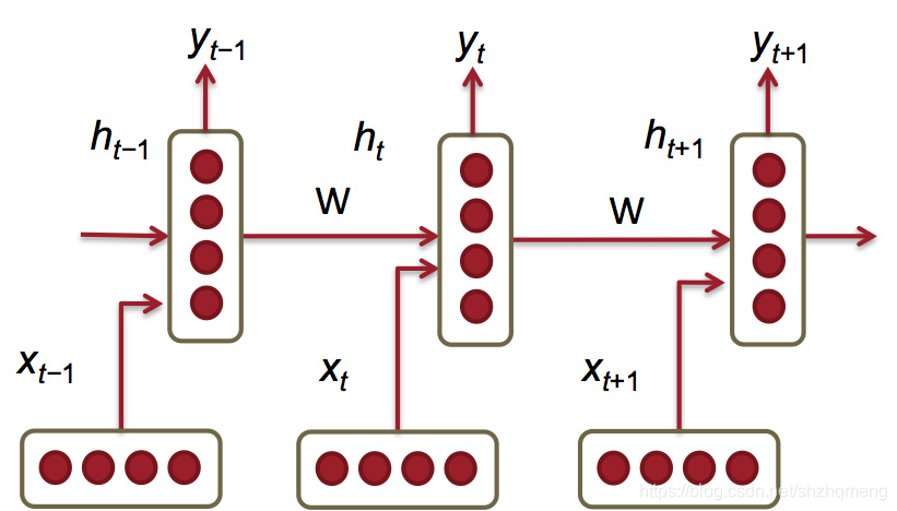
这种思路非常清晰,这里就不赘述了。思路就是序列根据前面的序列预测下一个。
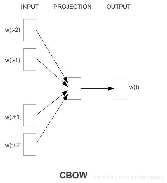
基于CBOW的方法
CBOW的思路是通过两边预测中间的词。图中的SUM函数就是我们在准备中介绍的向量化计算。
w
(
i
)
w(i)
w
(
i
)
就是文字数字化的输出。
class WordEmbedding:
    def __init__(self, embeding_size, vocabulary_size, window_size):
        self.__graph = tf.Graph()
        self.__session = tf.Session(graph=self.__graph)

        self.__embeding_size = embeding_size
        self.__vocabulary_size = vocabulary_size
        self.__window_size = window_size
        self.__epoch_num = 10
        self.__embedding = None


    def embedingInit(self, vocabulary_size, embeding_size, x_onehot):
        embedding = tf.Variable(tf.random_uniform([vocabulary_size, embeding_size]))
        self.__embedding = embedding
        x_vec = tf.nn.embedding_lookup(embedding, x_onehot)
        return x_vec

    def graphCreate(self, x_vec):
        hidden_state = tf.reduce_mean(x_vec, axis=1)
        weight = tf.Variable(tf.truncated_normal(shape=[self.__embeding_size, self.__vocabulary_size]), dtype=tf.float32)
        bias = tf.Variable(tf.truncated_normal(shape=[1, self.__vocabulary_size]), dtype=tf.float32)
        y_logit = tf.matmul(hidden_state, weight) + bias
        y_softmax = tf.nn.softmax(y_logit)
        return y_logit, y_softmax

    def calculateLoss(self, logits, labels):
        cost_array = tf.nn.sparse_softmax_cross_entropy_with_logits(logits=logits, labels=labels)
        return tf.reduce_sum(cost_array)

    def create_graph(self, batch_size):
        with self.__graph.as_default():
            self.__batch_size = tf.placeholder(dtype=tf.int32, name='batch_size')
            self.__x_ids = tf.placeholder(dtype=tf.int32, shape=[None, self.__window_size * 2], name="x_ids")
            self.__x_labels = tf.placeholder(dtype=tf.int32, shape=[None], name="x_lables")
            x_vec = self.embedingInit(self.__vocabulary_size, self.__embeding_size, self.__x_ids)
            tf.add_to_collection("infer", x_vec)
            y_logit, y_softmax = self.graphCreate(x_vec)
            cost = self.calculateLoss(y_logit, self.__x_labels)
            return cost, y_softmax


    def train(self, batch_sample, batch_label):
        batch_size = len(batch_sample[0])
        cost, y_softmax = self.create_graph(batch_size)
        with self.__graph.as_default():
            train = tf.train.AdamOptimizer().minimize(cost)
            self.__session.run(tf.global_variables_initializer())

            for i in range(self.__epoch_num):
                index_array = np.arange(len(batch_label))
                random.shuffle(index_array)
                for index in index_array:
                    if (len(batch_label[index]) != batch_size):
                        continue
                    _, lost_value = self.__session.run([train, cost],
                                                       feed_dict={
                                                           self.__batch_size: batch_size,
                                                           self.__x_ids:batch_sample[index],
                                                           self.__x_labels:batch_label[index]
                                                       }
                                                    )
                    print(lost_value)

                save_path = tf.train.Saver(tf.trainable_variables(), max_to_keep=4).save(self.__session, "./data/model/model.ckpt")
                print(save_path)
	def infer(self, model_path):
		saver = tf.train.import_meta_graph(model_path + ".meta")
		with tf.Session() as sess:
			saver.restore(sess, model_path)
			y = tf.get_collection("infer")[0]
			graph = tf.get_default_graph()
			batch_size = graph.get_operation_by_name("batch_size").outputs[0]
			ids = graph.get_operation_by_name('x_ids').outputs[0]
			ret = sess.run(y, feed_dict={batch_size:[1], ids : [[2,3,4,5]]})